Rendering fundamentals built one way of rendering a location: compute the smooth field, percentile-stretch it, and map a palette across it. There are many other ways to render a fractal, each reaching for a different effect. A rendering mode is any recipe for turning a location's orbits into a picture. An orbit is a whole path through the complex plane, and escape time keeps just one number from it, so there's a lot left to use. Most modes work like smooth: reduce each orbit to a value, collect the values into a field, and hand the field to the same stretch and palette. Some don't. Some blend two renderings into one, one shifts the palette by where the orbit went, and some skip fields and paint the orbit's behavior directly, which is roughly the order they come in below.
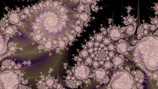
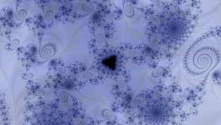
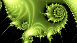
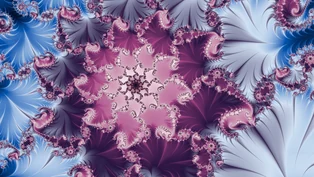
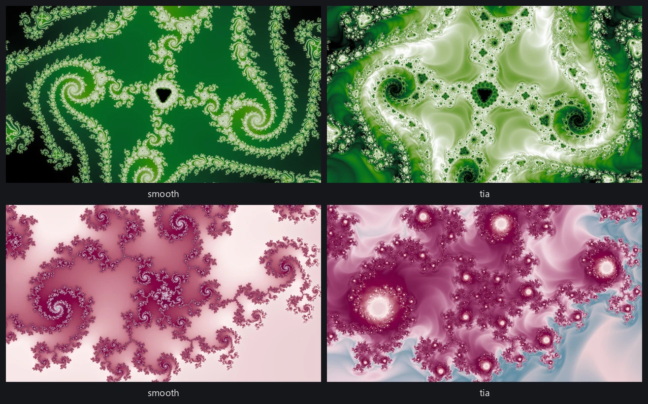
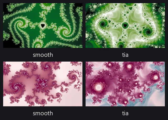
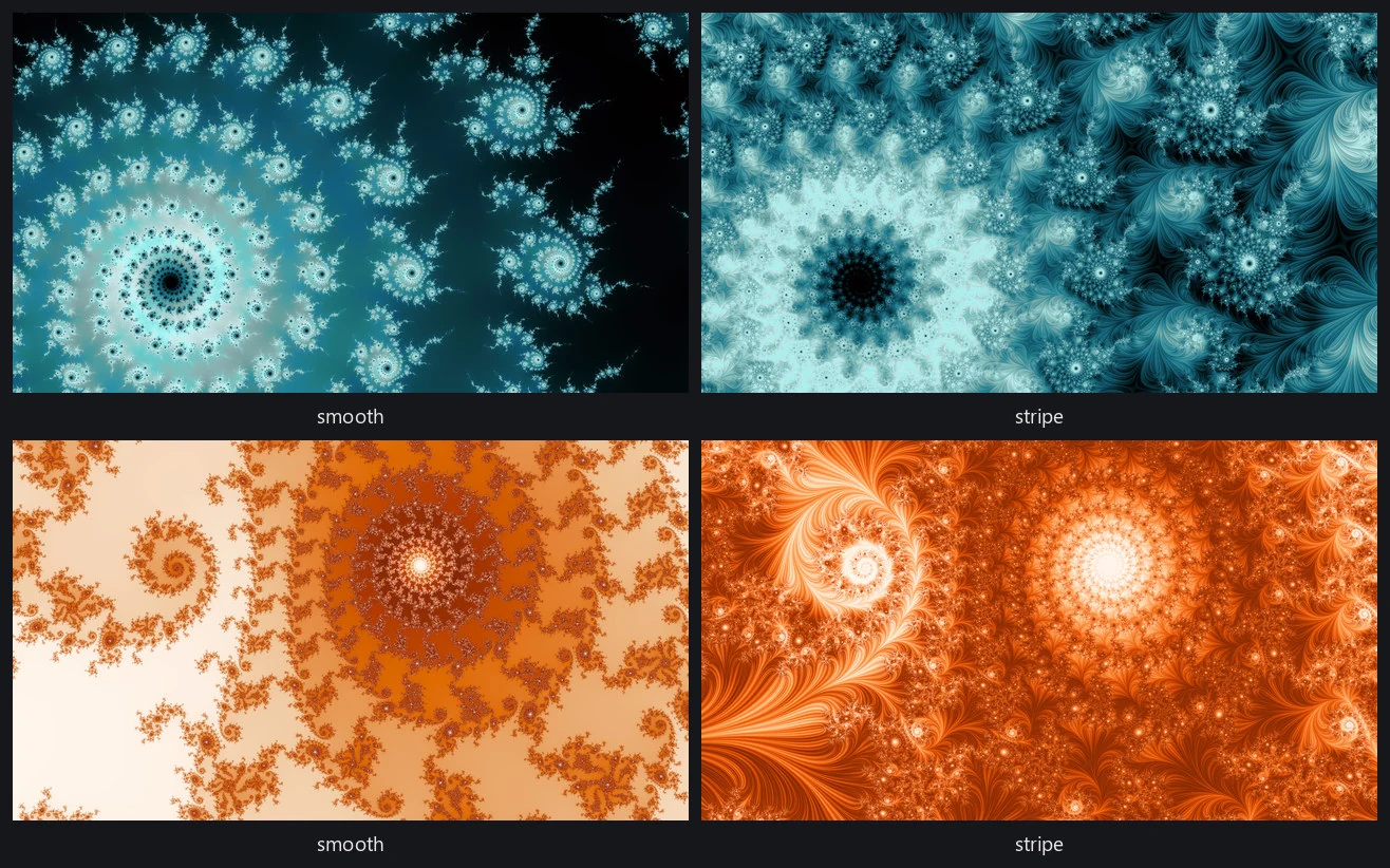
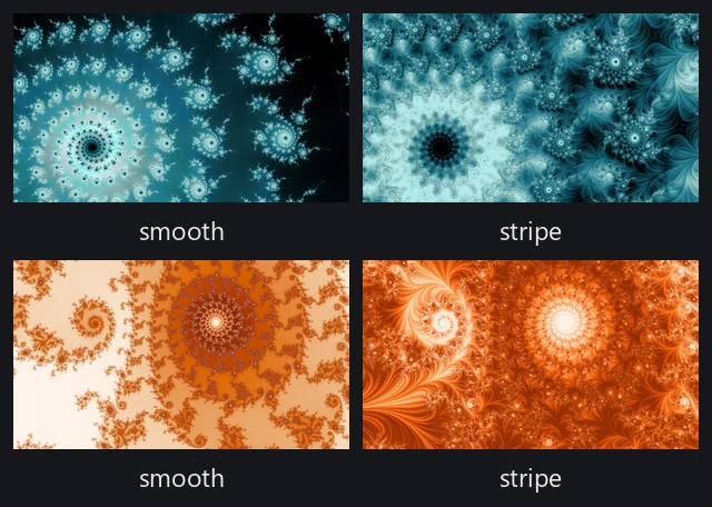
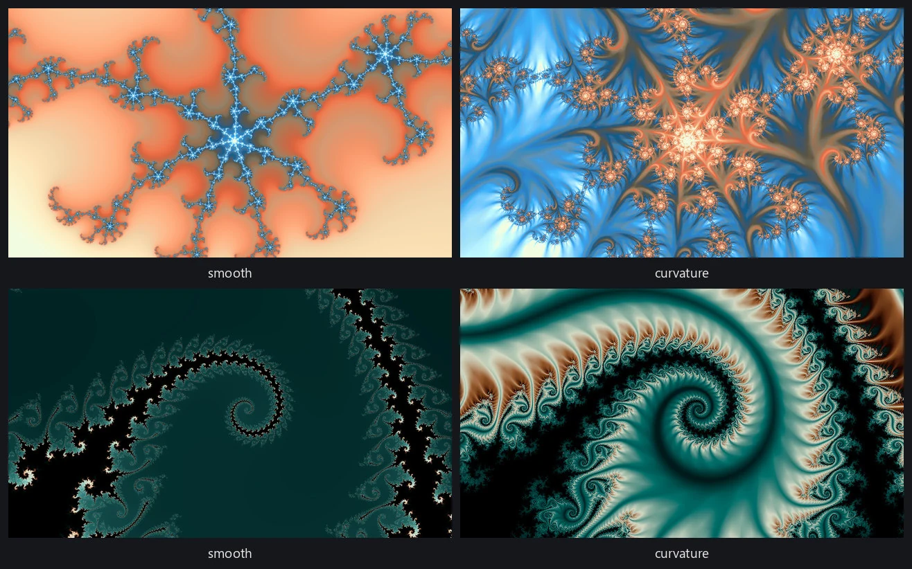
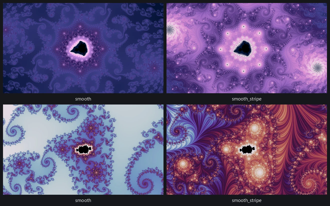
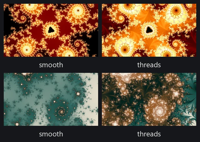
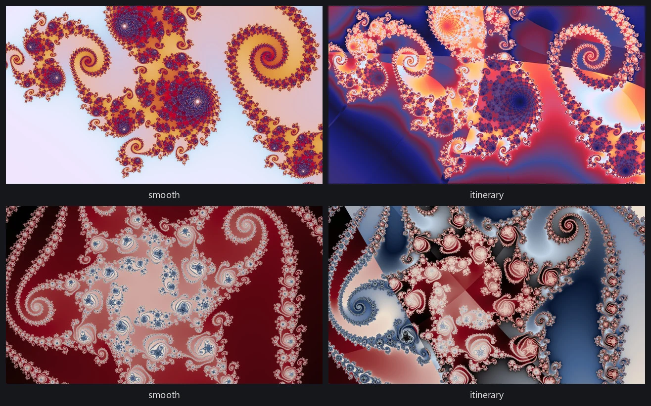
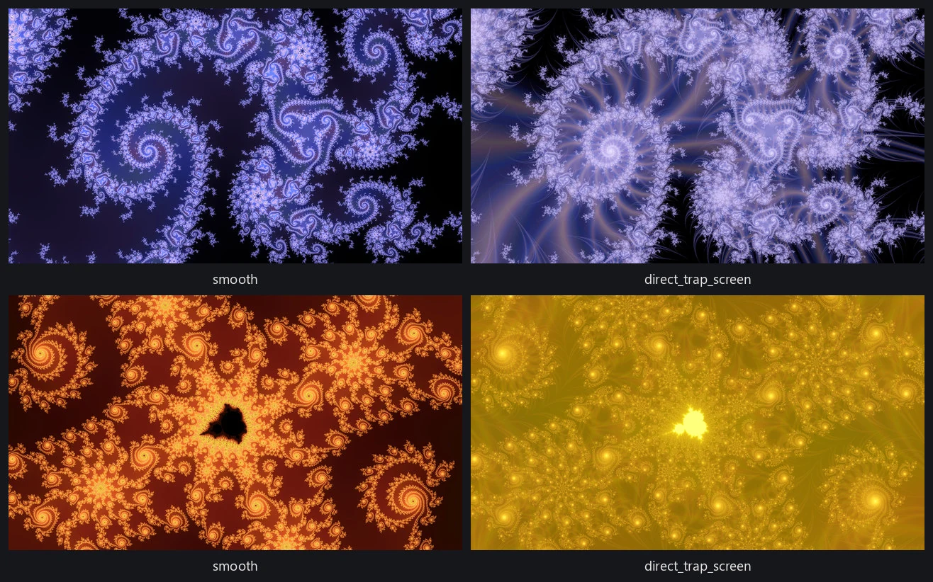
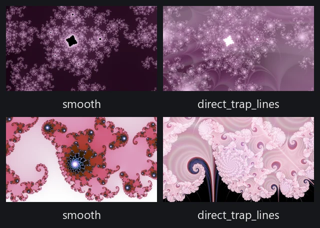
I tried a wide range of the techniques people have developed for these objects and kept my favorites, shown below. The rest of this page goes through them, with the rough parameter ranges I picked for each. Most figures show a location twice, smooth on the left and the mode on the right, in the same palette, so whatever changes between the panels is the mode.
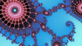
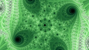
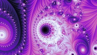
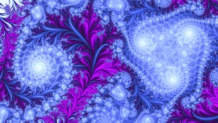
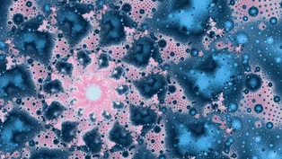
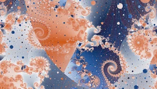
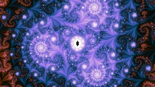
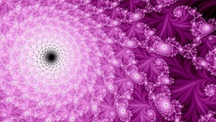
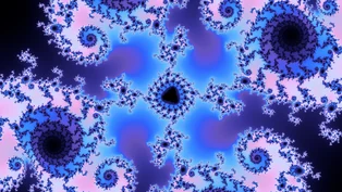
Fields from the orbit's path
Three modes keep smooth's recipe, one number per orbit and one continuous field, but measure the path instead of the clock.
Triangle-inequality average (tia) checks, at every step, where the orbit landed within the range it could have landed in. The triangle inequality brackets the next distance from the origin between a lowest and highest possible value, and the mode scores the real landing as a fraction between them, averaged over the orbit. Because that fraction can swing fully from one step to the next, the field bands far more finely than escape time: it reads as engraving where smooth reads as contour lines.
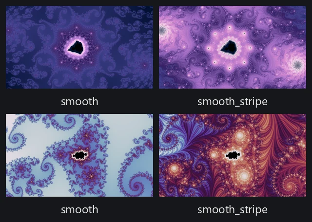
Stripe coloring works from the angles of the orbit's points. It averages a wave over those angles, one-half plus one-half the sine of six times the angle, where six is the stripe count the pipeline draws with. The crests show up as flowing bands laid along the fractal's structure. As with the other orbit averages here, the last term is blended in by the fractional part of the smooth count from rendering fundamentals, so crossing a whole escape step doesn't add a terrace of its own.
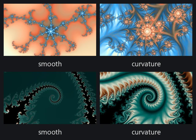
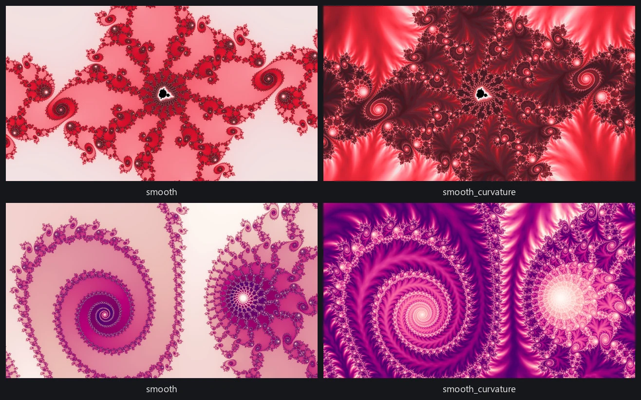
Curvature coloring measures how sharply the path turns: the unsigned angle between each step and the one before it, averaged along the orbit. Orbits that turn differently separate cleanly even when they escape at nearly the same moment, so the difference shows up where the smooth field has gone flat.
Orbit traps
An orbit trap places a fixed shape in the plane and asks each orbit how close it ever came to it. No trap is its own mode here. Traps appear as a texture over smooth in the composites, and painted directly in the last family on the page. Two shapes do that work. The cross trap is the distance to the two coordinate axes. The Gaussian-integer trap is the distance to the grid of points with whole-number real and imaginary parts, so one trap cell repeats across the whole plane, and the texture tiles like graph paper crumpled along the fractal's folds. Unlike every field mode above, a trap is defined for interior points too, which is how a trap texture fills the normally black lake with structure.
Blending modes together
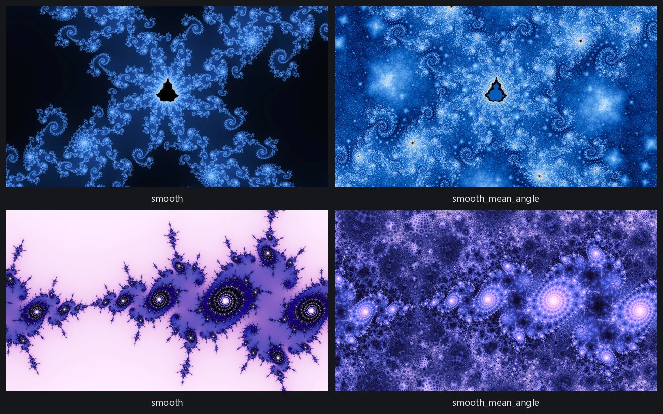
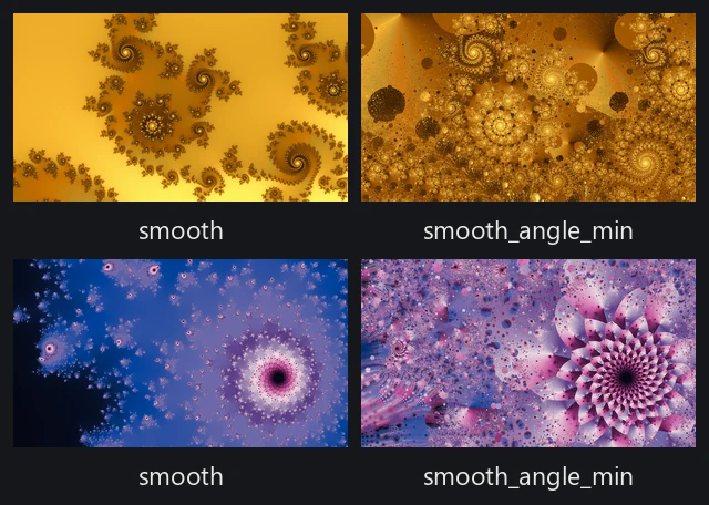
A composite is also a rendering mode. The engine renders the same location twice, a base and a texture, normalizes each, and blends them with a standard blending operator such as multiply, screen, or add. Five of the pipeline's modes are built this way, all on a smooth base, and four of them blend with screen at 85% strength. smooth_stripe and smooth_curvature lay their namesake fields over smooth. smooth_angle_min lays over the angle of the iterate at the orbit's closest approach to the Gaussian-integer trap. smooth_mean_angle takes the orbit's nearest, mean, and farthest distances to that same lattice and turns their imbalance into an angle, so it draws how lopsided the orbit's approaches were rather than where they came from. I picked 85% by eye: at full strength the texture's own normalization competes with the base's, and the escape structure underneath stops reading.
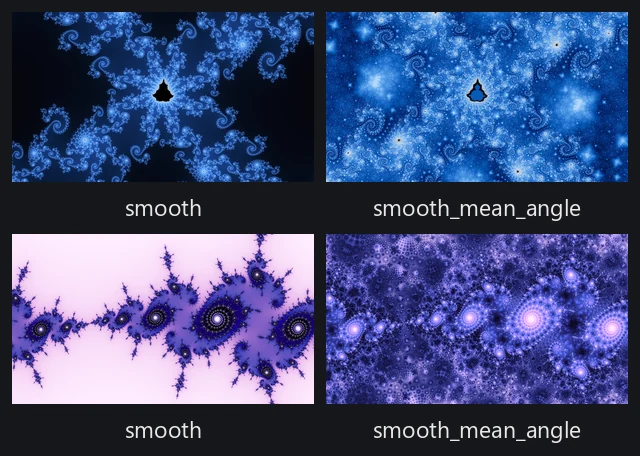
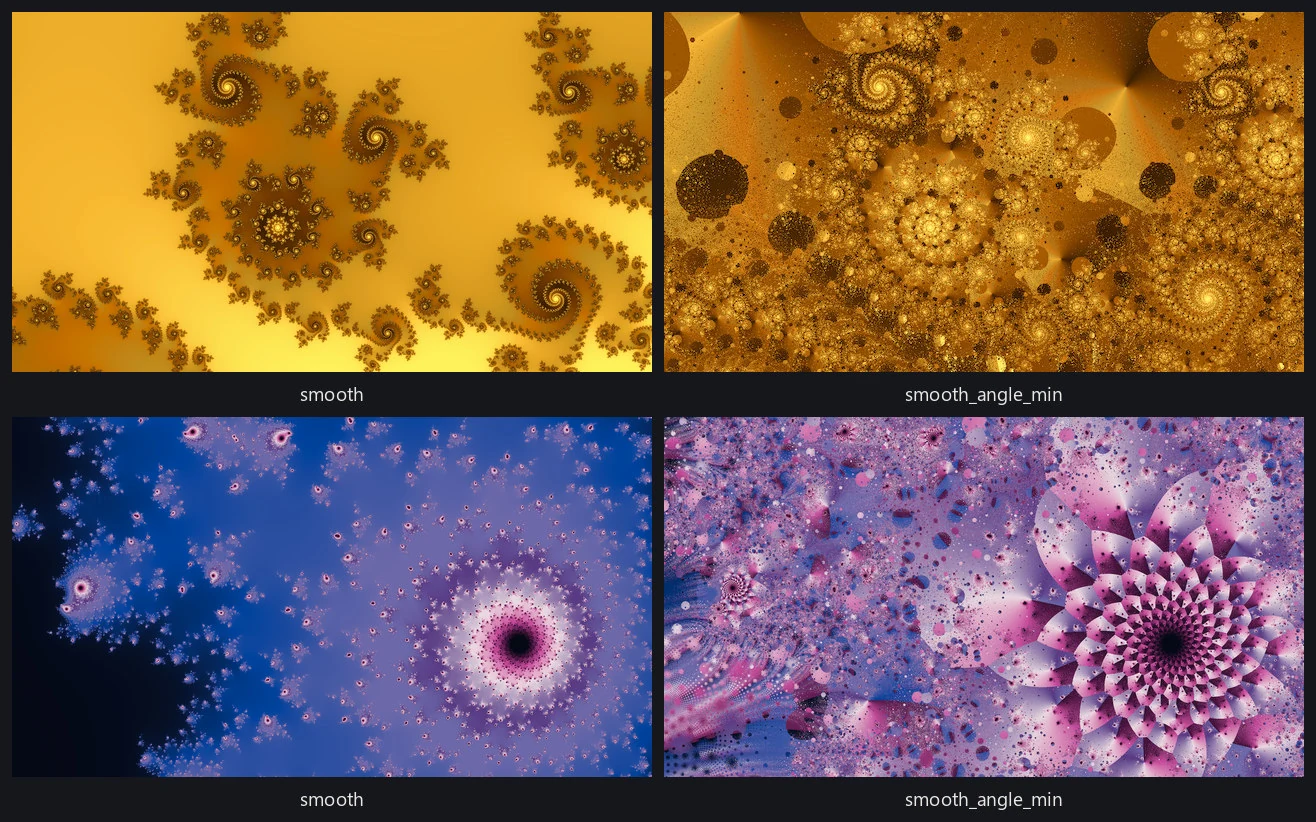
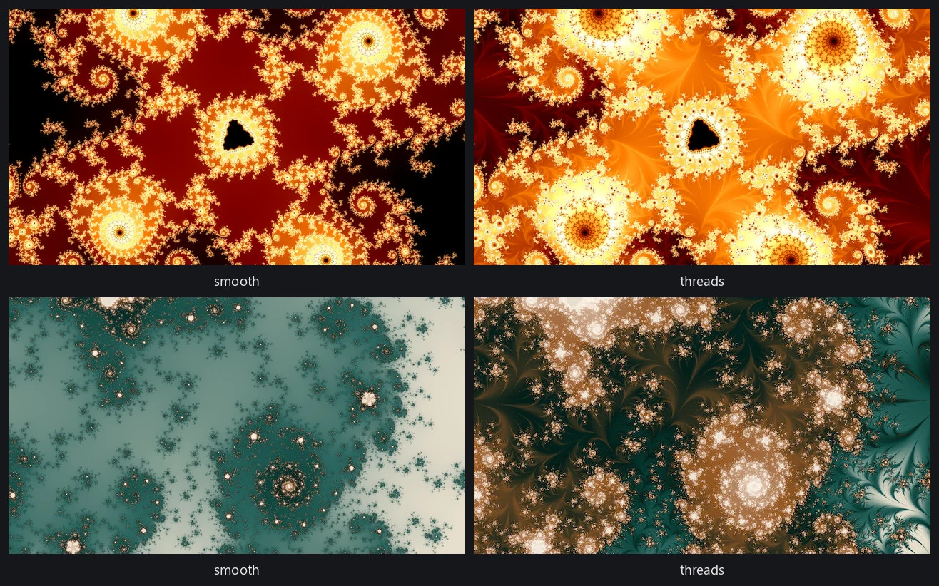
The fifth, threads, goes furthest. Its texture accumulates the cross trap over the whole orbit: every pass near the axes contributes, weighted by a narrow bell around the trap, so an orbit that grazed the axes a dozen times reads differently from one that grazed once. The texture is added over the smooth base at half strength, and the additive blend is why its sparse filaments glow on top of the classic rendering rather than mixing into it. It's also expensive, because the trap is evaluated on every iteration, so the cost lands hardest where orbits run longest.
The itinerary mode
The itinerary mode comes from a classical idea in dynamics: instead of asking when an orbit escapes, ask where it goes on the way. Cut the plane into four angular sectors around the origin, record the sequence of sectors the orbit visits, and read that sequence as base-four digits after the point, so the first few moves dominate the value and each later move refines it. The image splits into patches where every orbit opened with the same route, with hard edges where routes diverge, so it looks like stained glass where smooth looks like airbrush. The itinerary doesn't form a field of its own. Smooth is drawn underneath, and each pixel's address rotates its palette position by up to half a turn, so the patches appear as coordinated recolorings of the classic structure. On Julia sets, where every pixel is its own starting point, the route starts from the first iterate instead, or the leading digit would just cut the picture into quadrants.
Direct traps
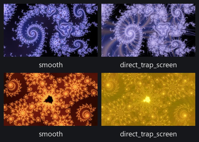
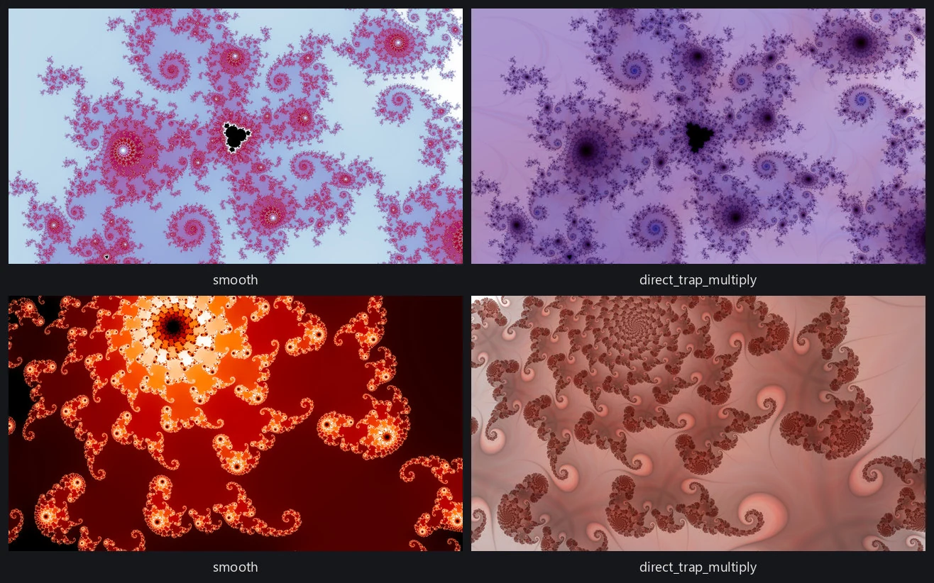
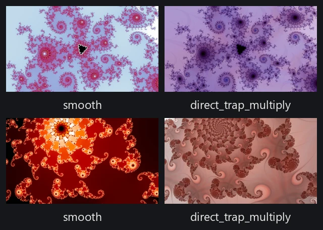
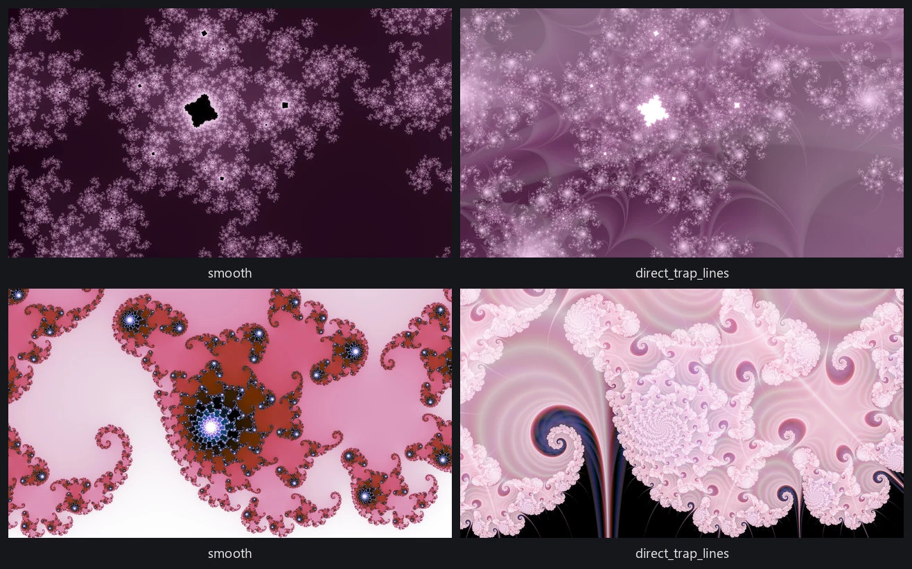
The last family never makes a field. A direct trap watches each orbit as it iterates, and whenever an iterate comes within a threshold of the trap shape, it samples the palette and paints that sample into the pixel right then. How close the iterate came decides both where in the palette the sample is taken and how much of it lands, which is why the strokes come out soft-edged with nothing extra to tune. A pixel's final color is the stack of every near-miss its orbit made, in order.
Three modes ship this way, from two shapes. The cross of the coordinate axes carries two of them, once brightening a black ground and once darkening a white one, and they read nothing alike. The third uses the real axis alone. Because nothing is normalized per frame, direct traps are the only modes that don't adapt to their location: where near-misses are sparse they're spectacular, and where they're everywhere the picture washes out.
The modes the pipeline draws
The search for good locations (finding good locations) only renders smooth. Every other mode enters in finding good wallpapers, when the pipeline takes a found location and renders it in several modes, drawn at random from the mined roster with none repeated, so no one mode takes all of that location's attempts.
I search over modes rather than picking one and using it everywhere, because a mode that's great at one location can fail badly at the next, even when the geometry is good. So I try several modes at every location and keep whatever survives. The table below shows how the judge rated every candidate the pipeline has rendered in each mode, across the four quality tiers from training judges, counting only locations whose smooth rendering it rates a three or better, so every row starts from geometry that works. These are the judge's scores, not mine, since nobody has looked at three hundred thousand pictures, and the judge runs optimistic compared to my ratings. Even so, most modes spend most of their attempts at a one or a two, and some, like direct_trap_lines, need about 25 attempts to find one strong result. I keep mining until even the modes with a lower hit rate leave enough strong candidates for the galleries. The last two columns are what an attempt costs: the engine time to render one candidate at the size the judge scores (640×360, supersampled 2×) and a finished wallpaper at full size (2560×1440, supersampled 3×).
| mode | q1 | q2 | q3 | q4 | candidates | candidate render | wallpaper render |
|---|---|---|---|---|---|---|---|
| smooth | 3% | 15% | 54% | 28% | 56,264 | 0.5s | 27.7s |
| tia | 8% | 29% | 45% | 18% | 62,418 | 0.8s | 57.3s |
| stripe | 17% | 28% | 37% | 18% | 56,757 | 1.4s | 2m56s |
| curvature | 49% | 35% | 13% | 3% | 18,737 | 1.1s | 1m42s |
| smooth_stripe | 15% | 29% | 41% | 15% | 12,870 | 6.2s | 3m06s |
| smooth_curvature | 28% | 38% | 27% | 7% | 11,913 | 4.5s | 1m14s |
| smooth_mean_angle | 39% | 33% | 19% | 9% | 14,883 | 5.1s | 2m25s |
| smooth_angle_min | 35% | 33% | 24% | 8% | 14,340 | 4.9s | 2m43s |
| threads | 5% | 24% | 49% | 22% | 12,274 | 3.0s | 51.5s |
| itinerary | 8% | 33% | 45% | 14% | 12,998 | 3.3s | 1m43s |
| direct_trap_screen | 33% | 42% | 19% | 6% | 12,261 | 1.4s | 1m22s |
| direct_trap_multiply | 40% | 25% | 29% | 6% | 23,716 | 2.0s | 19.5s |
| direct_trap_lines | 33% | 45% | 18% | 4% | 13,402 | 1.3s | 54.0s |
The candidate column is a mean over the candidates each row counts, and the wallpaper column is a mean over the finished wallpapers rendered in that mode. Times are for a single desktop CPU.
Beyond this catalog
The wider fractal-art world has many more ways to render these objects. A few come up often enough to deserve a pointer:
- Distance estimation tracks how sensitively each orbit's endpoint responds to nudging the pixel, and turns that into an estimate of the pixel's distance to the set's boundary. Drawn directly, the boundary becomes crisp filaments of uniform width at any zoom, like a technical drawing. The renderer implements it and will draw it on request; it just isn't among the modes the wallpaper search draws from.
- Normal-map lighting treats a field as terrain and lights it as relief, the same normal mapping trick games use. I left it out on purpose: it turns a fractal into an embossed metal plaque, replacing the picture's own structure with a lighting model's.
- The Buddhabrot drops per-pixel coloring entirely. It follows the full orbits of millions of escaping points and brightens every pixel they pass through, building something like an X-ray of where the dynamics travel.
- Histogram coloring maps field values by how often each occurs, so every color is used in proportion to how much of the image wants it. It solves the same squeezed-range problem as the percentile stretch, but reads the whole distribution rather than two points on it.
- Fractal flames leave escape-time fractals altogether. They iterate a system of nonlinear functions and accumulate the wandering point's path into a log-scaled density image, which is a different object with its own tools.
- Programs like Ultra Fractal treat all of this as an open library: thousands of user-written coloring algorithms, combined freely with any formula and stacked in layers.
One discovery, many wallpapers
Finding a good location is the uncertain part. Once I have one, I can render it in smooth, tia, threads, or any other mode, each in any palette, so one discovery becomes many possible wallpapers. Finding good locations covers how locations are found, training judges covers teaching a machine to recognize a keeper, and finding good wallpapers is where a location is drawn again and again across the roster on this page.